What is MS Excel

What is MS Excel, MS Excel (Microsoft Excel) is a spreadsheet program developed by Microsoft and helps users organize, analyze, and calculate data. It organizes data into rows and columns, allowing you to create mathematical functions, financial analysis, charts, and reports using numbers, text, and formulas.

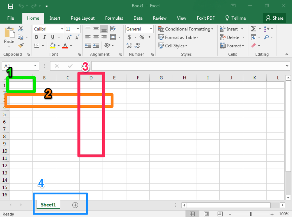
Introduction to Excel User Interface

Office Button – Under this option, there are options related to taking a new blank page, opening and saving the created file. This option is located in the File Menu in the 2010-2016 version. All the options of the Office button will be given to you below.
Quick Access Toolbar Any option can be added to this toolbar. Right click on the option you want to add and then click on Add to Quick Access Toolbar. Its advantage is that when you need an option repeatedly which you need to access from the menu, you will not have to go inside any menu but just click once.
Title Bar This part is the top line of the software which is called the title bar. It shows the name of your file which you keep saved.
Minimize / Maximize / Close

1. Minimize: With its help you can minimize and hide the open MS Excel.

2. Maximize: It is used to enlarge the open window. When it gets smaller in any way or maximize is clicked by mistake, then the screen gets smaller. At that time, on clicking maximize, it comes back to its full size.

3. Close is used to close MS Excel

Menu Bar All the menus of MS Excel are present in this bar. In which the Format menu and Developer menu are hidden. The Format menu becomes visible on clicking any picture or shape. But the Developer menu is shown by going to the Word option and from the Popular tab.
Ribbon – All the tools are present in it. Which contains tools related to font, paragraph, style.
Note This changes depending on the menu selection.
Name Box: Whatever your active account is, The cell will have its name visible as data.
Formula Bar – Inside this you will see the Excel formula which you insert in a cell, when you click on that cell, it will be displayed in the formula bar.
Scroll bar: With its help, the page can be moved up and down, right and left.
Sheets Through this you can insert sheets in your Excel and can change the name, color etc. of your sheet by clicking the right button of the mouse on any sheet.
Status Bar In this you will get options for view style and zoom in and zoom out. Description of Office Button

Description of Office Button

1. New Ctrl+N This option is used to bring a new blank document.
2. Open Ctrl+O This option is used to open old files or previously saved files.
3. Save Ctrl+S This option is used to save the current file.
4. Save as F12 This option is used to save the saved file with a different name in another drive.
5. Print Ctrl+P This option is used to print the prepared page.
6. Prepare In this you will get options like properties, encryption, and digital signature.
7. Send is used to send the current file.
8. Publish is used to publish on the internet or server.
9. Close is used to close the currently open page.

Description of Home Menu

1 Clipboard Under this option, Cut Copy Paste and Format Painter are present, which have different functions, which can be read in detail below.

1. Cut: Through this, any text, picture or shape can be cut and kept in the clipboard which can be pasted and inserted in MS Word. The cut shape, picture or text should remain selected and when it is cut, it moves away from there and goes to the clipboard.
2. Copy Before copying any text shape or picture, it must be selected and after copying it goes to the clipboard and it remains present on the page and also comes in your clipboard which is brought to the page during pasting.
3. Paste: Any text, picture or shape cut or copied above is used to paste. Paste Special is also present inside Paste, in which any object, text or shape copied from any other software is pasted. Paste As Hyperlink is used to paste like a hyperlink.
4. Format Painter Format painter is such a tool which is very useful. It is used only to copy the formatting inside the text, which increases your working speed. In this, if you have to change the font, change the color, change the size of a text again and again to make it the same way, then you can get relief in such a situation. In which format do you have to do all the text or just a part of it, then first select the way you want to do it and then click on Format Painter. As soon as you click, your cursor will become like a brush and on selecting the text, the same format will come on the selected text.

2 Under the Font dialog box, there are options to change fonts, font styles such as bold, italic, underline, increase or decrease font size, change font color and change underline color. You can read about them in detail below.

Font: With its help, we can change the style of the selected text or paragraph.
Font Size: It is used to increase or decrease the size of the text. If you want to use it to increase or decrease the size of a single paragraph or word, first select it and only then change the font size.
Bold Ctrl+B is used to make the selected text bold.
Italic Ctrl+I is used to italicize the selected text.
Underline Ctrl+U is used to underline the selected text.
Borders/Draw Borders Through this, you can add borders to your Excel sheet. By adding this, the rows and columns of your sheet become visible in the print preview, i.e., it will also be printed. If you do not add borders, then your page will be printed as a plain page.
Fill Color: Its help is used to fill color in the selected cells. Even if you select and fill multiple rows and columns at once, your filling will be done.
Font Color: With its help, the selected text or paragraph can be colored in any color.

3 Alignment Inside this you will get 9 options which are related only to alignment, read in detail below-

Top Align This option is used to top align the text written in a cell i.e. at the top vertically. Middle Align This option is used to center the text written in a cell vertically.
Bottom Align: This option is used to bottom align the text written in the cell i.e. to make it at the bottom vertically.
Orientation is used to set the text written in the cell at different angles
Align text Left: This option is used to move the text written in the cell to the left side, although the left side is already set.
Center: This option is used to center the text written in a cell.
Align text Right: This option is used to move the text written in the cell to the right side.
Increase Indent / Decrease Indent: With its help, you can increase or decrease the indent in Excel. It increases the spacing from the left side. You must have used it while writing a letter in MS Word.
Wrap Text: With the help of this option, you can display the text written in your cell in multiple lines. When a text is longer than the cell width, then this option is used so that the text wraps and automatically generates another line and appears in it.

4. Merge & Center Under this option, you will get 4 options which are as follows-

1. Merge & Center The job of Merge is to make multiple cells one, and the job of Center is to center your text align, in this both options are being used at once
2. Merge Across can also be done using this option This is done but there is a slight difference in it, when you use this option then it will merge from left to right only and not the entire selection. Note: This is used only to merge cells from left to right, it does not merge from top to bottom.
3. Merge Cell It is also used to merge and It is like center but it will only merge, the align will not change, in the previous option the align would also become center but not in this
4. Unmerge: It is used to unmerge cells that have been merged in any way.

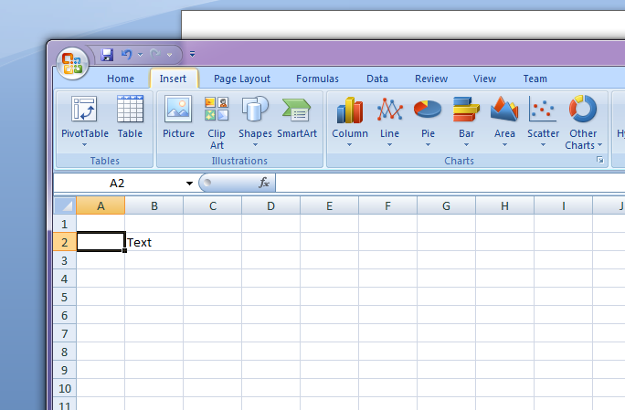
Description of Insert Menu

1. There are 2 options inside the Table dialog box, first is Pivot Table and Second table whose function is as follows-

Pivot Table: With the help of this option, you can insert a Pivot Table in your Excel sheet. It is an interactive table that provides the facility to analyze any Excel data easily and prepare large data in small and tabular form and it can sort, count and total (SUM) the data.
Table: Through this, one or more tables are used to insert and draw on the page.

2. Illustrations: Inside this dialog box, you will find five options, which include Picture, Clip Art, Shapes, and Smart Art, whose use is as follows-

Picture it through your sheet It is used to insert pictures like JPG, PNG and BMP.
Clip Art: This is also a picture but it is smaller in size. Which is already provided by the company.
Shapes: Shapes are used to insert lines, basic shapes, block arrows, flowcharts, callouts, stars and banners. Apart from this, you can also draw it yourself and add the desired color to it.
Smart Art Smart art is a shape which is used to show communication. In this you can use graphical list and any process to insert such as diagram. After inserting you can type any word in it.

3. Chart: All the options in this dialog box are used only for inserting charts, which helps you in understanding your data easily. In this, you can use many types of charts and give the desired design.

4. Links There is only one option in this which is What is a Hyperlink? Use it in Excel Any software is used to attach files to the sheet, which works like a link. Which can be followed by pressing Ctrl+click. If you insert a picture, it will open on Internet Explorer or in the default browser.

5. Text In this group, you will get 6 options which are as follows –

1. Text Box: This is used to bring a stylized text box on the page. As soon as you click on it, your mouse cursor will change and then you can draw at the angle you want. You will also get this option in the Shapes option.
2. Header & Footer: Inside this, you will get many options. The main options are mentioned below. When you click on this, a menu named design will open, inside which you will get many options which you have read in MS Word –
3. Header: It can be used to write the title of the document, name of the text, or some message etc. in the header. This can be increased or decreased according to the page margin. Note Header (Top Margin) is located on the upper margin.
4. Footer: It can be used to write the title of the document, name of the text, or some message etc. in the footer. This can also be increased or decreased according to the page margin. Note Footer (Bottom Margin) is on the bottom margin Is situated.
5. Number It is used to put page numbers in the header or footer
Within which you will get many types of numbering formats which can be customized after inserting.
6. Word Art: This option is used to write stylish text.
7. Signature Line – This is used to add digital signature. But only Microsoft partners can use it.
8. Object is used to insert a file from some other software into MS Word. With the help of text from file, it is used to bring the text written in another file into the current file.
9. Symbol: Through this you can write the text in your Excel sheet which is not given in the keyboard like copyright sign, paragraph sign etc.

Description of Page Layout Menu

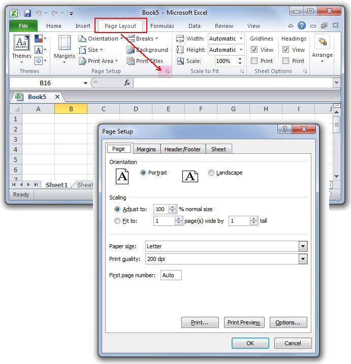
The Page Layout menu is used to do page-related settings. Which are as follows-

1. Themes – Under this, you can use it to change font style and color.
2. Margins are used to set margins according to the ruler. By default, one inch is set at the top, bottom, right and left. You can also set margins by customizing it yourself.
3. Orientation: With the help of orientation, the page is used to make it vertical (Portrait) and landscape. In this, portrait mode is set by default.
4. Size – With its help, it is used to size the document created or the new page taken, in which you can also add paper size yourself and by default letter size is set in it which is 8.5 inches wide and 11 inches long.
5. Print Area: Two options are given under this option, the first is Set Print Area, with the help of this you can set the print area so that only the selected part gets printed, the second option is Clear Print Area, its job is to remove the set print area.
6. Breaks– With its help, you can break the page, remove it and even reset it. It is used when some of our data is on the first page and some on the second page, then with the help of this you can put your data on a single page. For example, suppose you are writing a question and its four options in MS Word, you have written 5-6 questions and their options, in the eighth you have written the question but its option is going to the second page, then you would like that the question should also be on the second page, then you go to the starting point of the question which you want to adjust in the second page, then click on the break option. Similarly in Excel also, if your data is going to some other page, then break option is used for adjusting it.
7. Background: With its help you can put any picture in the background of your Excel sheet.
8. Print Titles – Through this you can print the address of the row and column given in Excel or else you can also hide it.
9. Scale to fit In this group you will get options related to setting the height and width of the print output in which you can set the size as per your requirement.
10. Sheet Options – Through this you can hide the headings and grid lines in Excel and if you want to print it, you can print it as well. If the print option is not ticked, then the headings and grid lines will not be printed.

11. Arrange In this group you will get options related to any (shape) object. Like-

1. Bring to Front 3-4 objects out of which object If you want to keep it on top, you can do so through this, similarly if you want to keep it at the bottom, you can do so through the Send to Back option.
2. Selection Pane This option is used when you have drawn many shapes, i.e. Objects You can then manage the object through the Selection pane like hiding, reordering and viewing the shape name etc.
3. Align: Align is used to make an object or an image left, right, center, top, middle and bottom.
4. Group is used to group two shapes. Group can be done only when two shapes are selected. Group option does not show on selection of a single shape. And any image cannot be grouped.
5. Rotate With the help of Rotate, you can customize your picture or object by going to 90 degree left, 90 degree right flip vertical, flip horizontal and more options.

Description of Formulas Menu

Inside this menu, you will find all the options related to formulas in which you can use different types of formulas and functions. Inside this, you will find 4 groups which are Function Library, Defined Names, Formula Auditing, Calculation respectively.

1. Function Library – In this group, you will find many types of functions, with the help of which you can easily do big math calculations like Financial, Logical, Text, Date & Time, Math & String etc.

Note You will understand all the functions given in this only if you use them one by one.

2. Defined Names Through this you can name the selected cell as per your wish. Then if you want, you can also write it in the formula, you can directly write the name you have selected. We have given the screenshot below in which name of A1 is Rakesh, name of A2 is Mgs and name of A3 is Rakesh Mgs. Active cell is A3 so Rakesh Mgs is visible in the name box but notice that Sum function is applied in the formula box next to the name box but in place of cell address the name of the cell which we have given directly is written but still the calculation is perfect, so similarly you can also change the name of any cell, and yes in the formula or function whether you input the cell address or input the name, both will work.

3. Formula Auditing – Through this group you can see on what a cell depends, you can indicate with an arrow those cells which are dependent on another or are taking data from another cell and you can also remove the arrow after seeing it. There is another option in this, Watch Window, with the help of which you can open a small window, as per your selection you can see the details of any cell like sheet, name, cell, value and formula. One advantage of this is that you can see that window from anywhere in Excel.

Calculation: With the help of this option you can turn auto calculation on and off.

Description of Data Menu

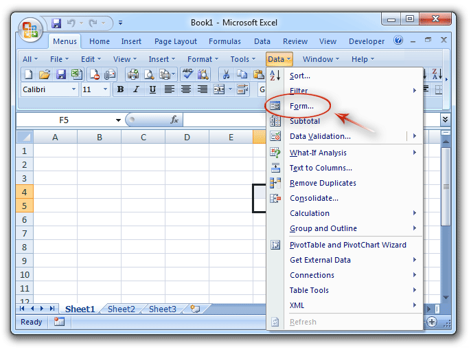
Under the Data menu, you can take data from any other software, add any URL from the internet and insert all the text inside it in your Excel sheet, inside this you will find 4 groups which are Connections, Sort & Filter, Data Tools and Outline respectively, its functions are as follows

An option is given before the connection group, whose name is Get External Data. With the help of this, you can insert data in your Excel from any other software like MS Access or any website or from any other source.

1. Connections Whenever we get data from “From Web” by inputting a URL in Get External Data, this option is used to set it. You can go inside the connection and check the properties.

2. Sort & Filter Through this, you can apply sort and filter option in your Excel, whose function is-

i. Sort To display your data in ascending order and descending order (A2Z, Z2A).
ii. Through filter you can view the data as per your wish, you can hide it if you want, you can view as much data as you need, when you apply it, a drop down button will be created in the first cell which will be selected, you can sort by clicking on it.

3. Data Tools In this, you are given 5 options which are as follows-

i. Text to Columns: This is used to divide simple text into multiple columns.
ii. Remove Duplicate This option is very useful in Excel, its job is to delete duplicate values. For example, if you are preparing a list and the data of a person is written as 2-3, then you select it and click on Remove Duplicate option and your duplicate data will be deleted.
III. Data Validation Through this you can apply validation to your Excel cell, if you do not know what this validation is then understand it, for example suppose we have to write a number from 10 to 50 in cell A5 and you have applied validation, then as soon as you write a number above 50 or a number more than this it will show you an error, similarly if you write less than 10 also it will show you an error.
iv. Consolidate Through this you can merge different cell ranges into one range.

4. What if Analysis – In this you will get 3 options whose functions are as follows- Through this you can fix something in your excel sheet

1. Scenario Manager is used to show its values.Through this you can fix something in your excel sheet
ii. Goal Seek: This is a very good option given in Excel, with the help of this you can know the unknown number, for example, suppose your exam is going on and you have one paper left, all the others have been completed, you have added the marks as per your wish that we got this much in this subject, similarly you have done all the calculations, now you need 80% but you don’t know how much marks you will get in the last paper so that 80% will be completed, this is used to know the number.

5. Outline Under this group, 3 options are given which are as follows-

i. Group With its help, you can group your selected cells.
ii. Ungroup With its help, you can use it to ungroup grouped cells

Subtotal is used to subtotal or sum the selected cells and it is automatically inserted according to its row.

Description of Review Menu

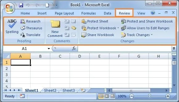
Inside the Review menu, you will find 3 groups, namely Proofing, Comments, Changes, whose functions are as follows-

1. Proofing This group contains commands related to word and text. Important commands in it are Spelling & Grammar. Which is used to view and correct the spelling and grammar errors in any word or paragraph text written in a cell. In this, Thesaurus option is used to find synonyms and antonyms of a word. And using Translate command, you can also translate text in different languages present in MS Office. You can select the text which you want to translate and click on Translate and then select the language in which you want to translate.

2. Comments When you want to write the meaning of a word or comment on a word, then we use comments. All the options related to this are given with the help of which you can modify the settings of comments.

3. Changes This group is used to protect your data in Excel, and you can lock your sheets and workbooks by putting a password so that no one can make any changes in your sheet, inside this you will get the option of sharing as well as Allow Users to Edit range, with the help of which you can select more than one user in your computer so that that user can make some changes in your data. After this, under Track Changes comes Highlight Changes, when you turn it on, then if any user makes any changes in your document, you will know, it will be highlighted and you can see what all has been changed in your file, this is called For accepting and rejecting, it has Accept and Reject Commands. By using the Accept Command, the changes made in the document are accepted (i.e. adding the changes to the document). And by using the Reject Command, the changes are not included in the document.

Description of View Menu

1. Workbook Views In this, you can set the way you want to see your workbook. By default, there is a normal view, if you click on page layout, then your sheet will appear as different pages in which you will also see header and footer, you can manage that too. Similarly, it is used to see in different previews.

Show/Hide option is given before the zoom group through which you can hide or bring the formula bar, gridlines, and headings. By default all these are shown.

2. Zoom You can zoom in on your sheet using all the options provided in it. 3. Window The following are the functions of the options provided in it-

3. Window The functions of the options given inside it are as follows-

New Window – Through this, you can open the currently open sheet in another window, while both the windows will remain the same. Then whatever changes you make in the open window, those changes will be visible in your original window as well.
Arrange All: It is used when two or more Excel workbooks are open and you are typing something by looking at another workbook or are mixing some data. When you click on it, a small dialog box will open in which you can set the type of view you want like Tiled, Horizontal, Vertical and Cascade as per your requirement. You must try it once so that you can understand it well.
Freeze Panes – this option is very useful in Excel, it comes in handy when you make any kind of list in Excel like serial number, someone’s name, address, contact details etc. Then what happens is that after maximum 30 rows you will have to scroll due to which the headings written above like serial number, someone’s name, address, contact details etc all get hidden, then you can lock it using this option so that it remains stable at one place. In this you can freeze all the rows and columns together or you can do it even if you want to freeze only the rows or columns, try this also once, only then you will understand.
Save Workspace: Through this, you can save the layout you are currently using on your hard disk. That is, if you have created a custom view as per your requirement, then you can save it forever so that you don’t have to create the view again next time.
Switch Workbook: This option is used to switch more than one open workbook through a switch. As soon as you click on the switch, you will see an option that will have the title of all your open workbooks. On clicking it, you will go to the same workbook on which you have clicked.

4. Macros This is a VBS (Visual Basic Script) program which apart from Excel is also available in MS Excel, Photoshop, CorelDraw. This option is very good, through it you can do any big work in a few seconds, it records your activities like suppose you are making the result of weekly test in Excel and in it you have written the number of all the weeks (of a student), after that you can go to macros and turn on recording, after that add all the marks which it records, then when all the marks are added then stop recording so that the recording gets saved, and then when you write the number of any other student then run the recorded macro, your total will become automatic.

Note: You will find all the options related to this in the Developer menu which remains hidden. To enable it, you can enable it by ticking on Show Developer in the Ribbon in Popular in Excel Options.

Follow on Instagram:

Follow on Facebook page:

MS Excel